“What I cannot create, I do not understand”
And reimplementing the wheel is something I really do love to do: it is maybe the best way to really understand those concepts in depth.
But I do not only like to build things that work, it even better when one can also make complex things simple so that they can then better be understood, extended or redesigned.
And here, this is not something that is studied by machine learning generally: this is software design, and software engineering.
I decided to create a small library to easily play with all those notions.
I call it joml, which basically mean “joml One More
Layer”1.
Let’s go through the design and the process of creating, and training Neural
Networks using this toy library: this will also introduce the way joml has been designed.
Notations and definitions
Before diving in the details of the training procedure, let’s present some
notations. As well as a general overview on the way networks things are
implemented in joml.
Network and layers
Let’s note $\mathcal{N}$ a neural network. As you know, this network consists of several — and possibly different — Layers.
For now, we will only stick to FullyConnected layers which will simply be referred to as Layer in what follows. Such layers can be abstracted to allow extending this notion and define new type of layers.
Typically a Layer, is nothing more than a collection of neurons, that is a collection of weights and biases embedding an activation function.
For a given neuron $i$, if we note $\omega_i$ its vector of weights, $b_i$ the bias and $x$ the vector to operate on ; considering vectors as columns we have the value $z_i$ of the result of those two operations:
\begin{equation} \label{transfo} z_i = \omega_i^\top x + b_i \end{equation}
What neural networks mainly consist in is stacking Layers together, but before doing it, we have to use something that binds this results — otherwise stacking as many layers directly would result in just a linear transformation that is a simple Layer as far as we have them been defined, see the Bonus Track at the end for a quick example of this.
To bind those results, each neuron uses a non-linearity that is function $\sigma:\mathbb{R}\mapsto\mathbb{R}$ with nice property. Such a function is also called an activation function, which is defined bellow. So instead of $z_i$ being the output of the neuron $i$, we do have $a_i$ that is simply:
\begin{equation} a_i = \sigma(z_i) \end{equation}
If we generalise it at the scale of the Layer by introducing the vector of bias $b$, and the matrix $W$ whose $i$-th row correspond to the weights of the $i$⁻th neurone, we have — assuming that the $\sigma$ in \eqref{output} is simply the broadcasted version of $\sigma$ on a whole vector.
\begin{equation} \label{output} a = \sigma(W x) + b \end{equation}
Finally, if we note $L$ the number of its layers. We can for each layer $l\in {1,\cdots, L}$ note $W^{(l-1,l)}$ the matrix of weights used in the transformation from the previous layer $l-1$ to this considered $l$ layer; we also note $b^{(l)}$ the vector of biases of this layer. The equivalent of layer $0$ corresponds to the input $x$ and has no associated weights nor biases.
Hence, if we note $N_l$ the size of the layer $l$, we have by construction:
\begin{equation} \forall l \in {1,\cdots, L},\quad W^{(l-1,l)} \in \mathbb{R}^{N_l\times N_{l-1}},\quad b^{(l)}\in \mathbb{R}^{N_l} \end{equation}
Thus, a Layer $l$ is entirely specified using a size $N_l$, an activation function $\sigma_l$, and a pair of parameters $(W^{(l-1,l)}, b^{(l)})$.
In joml, this concept is implemented under the Layer
class. A
Layer wraps a matrice of weights and biases as well and also embeds
optimizers and information about a previous Layer. Some caches are also
needed for the training procedure.
Finally, we can define a network $\mathcal{N}$ as an ordered collection of $L$ layers, with an input size $N_0$. It can be seen as a function $\mathcal{N}: \mathbb{R}^{N_0} \to \mathbb{R}^{N_L}$ defined as:
\begin{equation} \mathcal{N} : x \mapsto \sigma_L\left(W^{(L-1,L)} \sigma_{L-1}\left(\cdots \sigma_1\left(W^{(0,1)} x + b^{(0)}\right) \cdots \right)+ b^{(L)}\right) \end{equation}
Prediction
For a vector $x^{(j)}$ , we define $\mathcal{N}(x^{(j)})$ as its prediction and we note it $\widehat{y}^{(j)}$.
\begin{equation} \widehat{y}^{(j)} = \mathcal{N}(x) \end{equation}
In the end, we will be comparing it to the real value of the mapping of $x^{(j)}$ that we will note $y^{(j)}$.
In joml, a network is implemented under the Network
class.
It basically wraps Layers and define generic methods to perform all the steps
that are deleguated to them.
Activation functions
Activation functions are functions that are used in Layer to perform a
non-linear mapping on the result of the transformation given in $\eqref{transfo}$.
The sigmoid function — denoted $s$, see equation \eqref{sigmoid} — used to be the canonical activation function used in neurons — as it was a really smooth function (it belongs to $C^\infty$), whose derivate — $s’$ given in \eqref{dersigmoid} — is quite nice.
\begin{equation} \label{sigmoid} \begin{matrix} s &:& \mathbb{R} &\to& [0, 1] \ & & x &\mapsto &\frac{1}{1+e^{-x}} \end{matrix} \end{equation}
\begin{equation} \label{dersigmoid} \begin{matrix} s’ &:& \mathbb{R} &\to& [0, 1] \ && x &\mapsto &s(x)(1 - s(x)) \end{matrix} \end{equation}
Now, people tend to only use ReLu, as the activation functions.
ReLu can be defined as a scalar function:
\begin{equation} \begin{matrix} \text{ReLu} &:& \mathbb{R} &\to& \mathbb{R}^+\ && x &\mapsto& \max(0,x) \end{matrix} \end{equation}
It is a simple (but not bijective) activation function whose derivative is:
\begin{equation} \begin{matrix} \text{ReLu}’ &:& \mathbb{R} &\to& \mathbb{R}^+\ && x &\mapsto& \left\{\begin{matrix} 1 & \text{if } x \geq 0\ 0 & \text{otherwise} \end{matrix}\right. \end{matrix} \end{equation}
Generally, activation functions are seen as their broadcasted version on vectors and matrices. That is in the case of ReLu:
\begin{equation} \begin{matrix} \text{ReLu} &:& \mathbb{R}^n &\to& \left(\mathbb{R}^+\right)^n\ &&&&\ && x &\mapsto& \left(\begin{matrix} \text{ReLu}(x_1)\text{ReLu}(x_2)\vdots\text{ReLu}(x_n) \end{matrix}\right) \end{matrix} \end{equation}
softmax is the function of choice when it comes to choose a modality over a set of multiples or to weight those modalities when given associate scorings in $\mathbb{R}$.
softmax is defined as:
\begin{equation} \begin{matrix} \text{softmax} &:& \mathbb{R}^n &\to& \mathbb{R}^n\ &&&&\ && x &\mapsto& \left(\begin{matrix} e^{x_1}\e^{x_2}\vdots\e^{x_n} \end{matrix}\right).\left[\sum_{i=1}^n e^{x_i}\right]^{-1} \end{matrix} \end{equation}
One could perform this choice between modalities only using an easier normalisation or not an hard max that would select the modality with the highest score, but the pros of softmax is that it is flexible and more appropriate when one has to make such choices with greater values 2. It also nicely pairs with a cost function as we are going to see.
In joml, the broadcast on the value of the function and on its derivative is
is performed via a template method on the ActivationFunction.value and
ActivationFunction.der: this way only the scalar values are to be
given for each new definition of an activation function; see the source code
of
ActivationFunction,
the one of
ReLu,
and the one of
SoftMax.
Cost Function
Cost functions, also called loss functions or objectives, are used to quantify the error that is to minimize to attain a goal.
Here, our goal is to correctly predict output of new data — so we want to minimize a dissimilarity we have between the predictions and the real values.
The most simple errors we could think of, is simply the mean absolute error, — abbreviated MAE — or the mean squared error — abbreviated MSE.
In fact, those can be used in the scalar case (think of predicting 0/1 only, or a scalar value only). But in the case of prediction between multiple modalities we need something else.
The cross-entropy, noted $H$, is defined on two probabilistic distributions represented here by the vectors $\hat{y}$ and $y$ as:
\begin{equation} \begin{matrix} H &:& [0,1]^K \times [0,1]^K &\to& \mathbb{R}\ & & (\hat{y},y) &\mapsto& - \sum_{k=1}^K \hat{y}_k \log y_k \end{matrix} \end{equation}
The cross-entropy measures the proximity of two probabilistic distributions: the smaller the cross-entropy of two probabilistic distributions is, the more similar those two distributions are.
It’s choice also makes optimizing the loss easy when using softmax.
We now have all the pieces to tackle the main pieces that is how to train neural networks.
Training procedure
The internals of the backpropagation algorithm are not described entirely here. Moreover, a vast variety of optimizers exists, Adam3 being a pretty robust one. Also, good notes of the theory are now available online.
All the art and engineering consists in finding a good set of pais of matrices of weights and biases ${(W^{(l-1,l)}, b^{(l)})}}$ so that an aggregation — the cost function — of similarities between pairs of vectors $(y^{(j)}, \widehat{y}^{(j)})j$ is minimized.
Let’s summarize the workflow of training a neural network. It breaks down in 5 steps:
-
Forward-Propagation: Each input $x\in \mathbb{R}^{N_0}$ gets forward-propagated in the network to get its output $\hat{y}\in \mathbb{R}^{N_L}$. For each layer $l$, its input $a^{(l-1)}$ as well as its affine transformation $z^{(l)}$ gets persisted ; \begin{equation} \left\{ \begin{matrix} z^{(0)} &=& x &\in \mathbb{R}^{N_0}\ a^{(l)} &=& \sigma_l(z^{(l)}) &\in \mathbb{R}^{N_l}\ z^{(l)} &=& W^{(l,l-1)} a^{(l-1)} + b^{(l)} &\in \mathbb{R}^{N_l}\ \hat{y} &=& a^{(L)} &\in \mathbb{R}^{N_L} \end{matrix} \right. \end{equation} Here, we do not just consider a single pair $(x,y)$, but generally $n$ pairs $(x^{(i)},y^{(i)})_{i=1}^n$.
See how this is performed in
jomlin aNetworkand in aLayer. -
Cost Evaluation: The differents outputs $\hat{y}^{(i)}$ of the inputs $x^{(i)}$ are then compared to their labels $y^{(i)}$: the cost for the cross-entropy is computed using the estimator given in equation \eqref{estimatorCost}. \begin{equation} \label{estimatorCost} \hat{H}\left({(\hat{y}^{(i)},y^{(i)})}{i \leq n}}\right) = \frac{1}{n} \sum_k \end{equation}}^n H(\hat{y}^{(i)},y^{(i)}) = - \frac{1}{n} \sum_{i=1}^n \sum_{k=1}^K \hat{y}^{(i)}_k \log y^{(i)
-
Back-Propagation: The error $\delta^{(L)}$ is calculated using $\nabla_{a^{(L)}}\hat{H}$, the gradient of the (estimated) cost $\hat{H}$ with respect to the vectors of outputs, $a^{(L)} \in \mathbb{R}^{N_L}$ (see equation \eqref{lastErr}) and is then back-propagated in the network 4. \begin{equation} \label{lastErr} \delta^{(L)} = \nabla_{a^{(L)}}\hat{H} \odot \sigma_L’(z^{(L)}) \end{equation} From here, the error $\delta^{(l)}$ associated to each layer $l$ can be calculated using the error $\delta^{(l+1)}$ associated to the layer $l+1$ using the recurrence relation \eqref{recurrenceRelation}. \begin{equation} \label{recurrenceRelation} \delta^{(l)} = W^{(l,l+1)\top} \delta^{(l+1)} \odot \sigma_L’(z^{(l)}) \end{equation} Each layer $l$ then persists its associated error $\delta^{(l)}$.
See how those two steps are performed in
jomlin aNetworkand in aLayer. -
Gradients calculation: For each layer, gradients of weights and biases get calculated using the persisted activation $a_l$ and persisted error $\delta_l$5. \begin{equation} \label{gradients} \left\{ \begin{matrix} \nabla_{W^{(l,l-1)}} \hat{H} &=& \delta^{(l)}\, a^{(l-1)\top}\ \nabla_{b^{(l)}} \hat{H} &=& \delta^{(l)}\ \end{matrix} \right. \end{equation}
See how this is performed in
jomlin aNetwork, in aLayerand in theSoftMaxCrossEntropyOutputLayer. -
Parameters update using gradient descent: A optimisation routine is then executed to update the weights and biases accordingly. Here a first order method — generally a variant of the gradient descent — is used to optimise each layer weights and biases. The simplest update is of parameters is done in equation \eqref{updateParam} \begin{equation} \label{updateParam} \left\{ \begin{matrix} W^{(l,l-1)} &\longleftarrow& W^{(l,l-1)} &-& \eta_l \nabla_{W^{(l,l-1)}}\ b^{(l)} &\longleftarrow& b^{(l)} &-& \eta_l \nabla_{b^{(l)}} \end{matrix} \right. \end{equation}
See how this is performed in
jomlin aNetwork, in aLayerand byGradientDescentand byAdam.
Running the wheel: a simplistic toy example
Let’s say that we are given a data set that represents a function that takes in
14 binary digits and output one of four numbers (${0,1,2,3}$), using joml
we can easily construct neural network to train to learn this function:
\begin{equation} f: {-1,1}^{14} \to {1,2,3,4} \end{equation}
The output vectors $(y^{(j)})_j$ are one-hot vectors, i.e vector such that:
\begin{equation} l_j = \left\{ \begin{matrix} (1, 0, 0, 0)^\top &\Leftrightarrow& f(x_j) = 1\ (0, 1, 0, 0)^\top &\Leftrightarrow& f(x_j) = 2\ (0, 0, 1, 0)^\top &\Leftrightarrow& f(x_j) = 3\ (0, 0, 0, 1)^\top &\Leftrightarrow& f(x_j) = 4\ \end{matrix} \right. \end{equation}
Let’s say that we want to construct three networks like this:
14-100-40-4 net: $1$ hidden layer of size $100$, $1$ hidden layer of size $40$ ($5704$ parameters)14-28x6-4 net: $28$ hidden layer of size $6$ ($4596$ parameters)14-14x28-4 net: $14$ hidden layer of size $14$ ($5940$ parameters)
each network having the cross entropy as the cost function on top of the softmax function for the training. All but the last fully connected layers have ReLU as the activation function.
Using joml, we can define those networks as follows:
import numpy as np
from joml.network import Network
from joml.layer import Layer, SoftMaxCrossEntropyOutputLayer

n1 = Network(input_size=14, name="14-100-40-4 net")
n1.stack(Layer(size=100))
n1.stack(Layer(size=40))
n1.output(SoftMaxCrossEntropyOutputLayer(size=4))


n2 = Network(input_size=14, name="14-28x6-4 net")
for _ in range(6):
    n2.stack(Layer(size=28))
n2.output(SoftMaxCrossEntropyOutputLayer(size=4))


n3 = Network(input_size=14, name="14-14x28-4 net")
for _ in range(28):
    n3.stack(Layer(size=14))
n3.output(SoftMaxCrossEntropyOutputLayer(size=4))
Training and Testing Set
The dataset used consist of all the elements of ${-1,1}^{14}$, namely 16384 vectors. $80\%$ of this space is used to train, the remaining $20\%$ of it to test.
| Train | Test | |
|---|---|---|
| Samples | $13107$ | $3277$ |
| Proportion | $80\%$ | $20\%$ |
To train those architectures, Adam have been used with the default parameters given in the original paper, that is $\beta_1=0.9$, $\beta_2=0.999$, $\epsilon=10^{-8}$ and a learning rate of $\eta=0.002$. We are using mini-batch of 32 example, and 10 epochs.
Using joml, performing the training on the 3 networks can be done with this snippet:
for network in [n1, n2, n3]:
    network.train(x_train, y_train)
    y_pred, y_hat, acc = network.test(x_test, y_test)
But one can also perform a benchmark with jolm to better see and understand
for network in [n1, n2, n3]:
    # Define a log file
    current_datetime = strftime("%Y-%m-%d-%H:%M:%S", gmtime())
    logs_folder = os.path.join("..", "logs")
    out_file = os.path.join(logs_folder,
                            f"benchmark_{network.name}-{current_datetime}.csv")

    # Benchmark the network
    logger = network.benchmark(x_train,
                               y_train,
                               x_test,
                               y_test,
                               csv_file_name=out_file,
                               num_epochs=10)

    # Dump results in a CSV file
    logger.dump_results()
    logger.plot_benchmark()
Results and discussions
Firstly the networks succeed to learn the given mapping $f:{-1,1}^{14} \to {1,2,3,4}$: test accuracies of more than $90\%$ are observed using the given procedure for all the networks (see the table bellow). The training cost is noisy: this is normal as we are using Mini-Batch instead of the entire dataset to train the network for one iteration.
| Architecture | Training Cost | Testing Cost | Training Accuracy | Testing Accuracy |
|---|---|---|---|---|
14-100-40-4 net |
0.0804 | 1.2273 | 1.0 | 0.9774 |
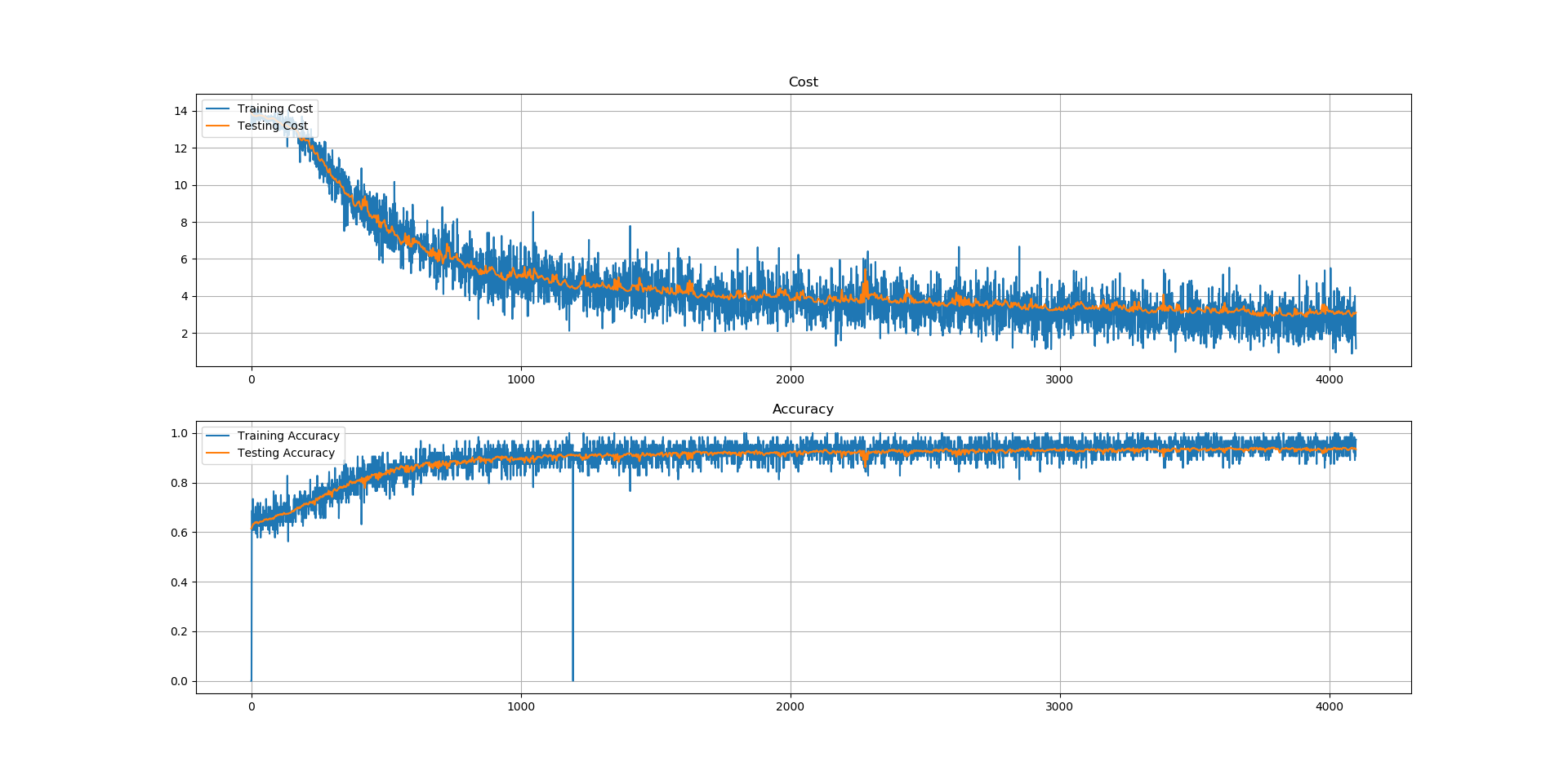
14-28x6-4 net |
5.3491 | 4.5165 | 0.8947 | 0.9150 |
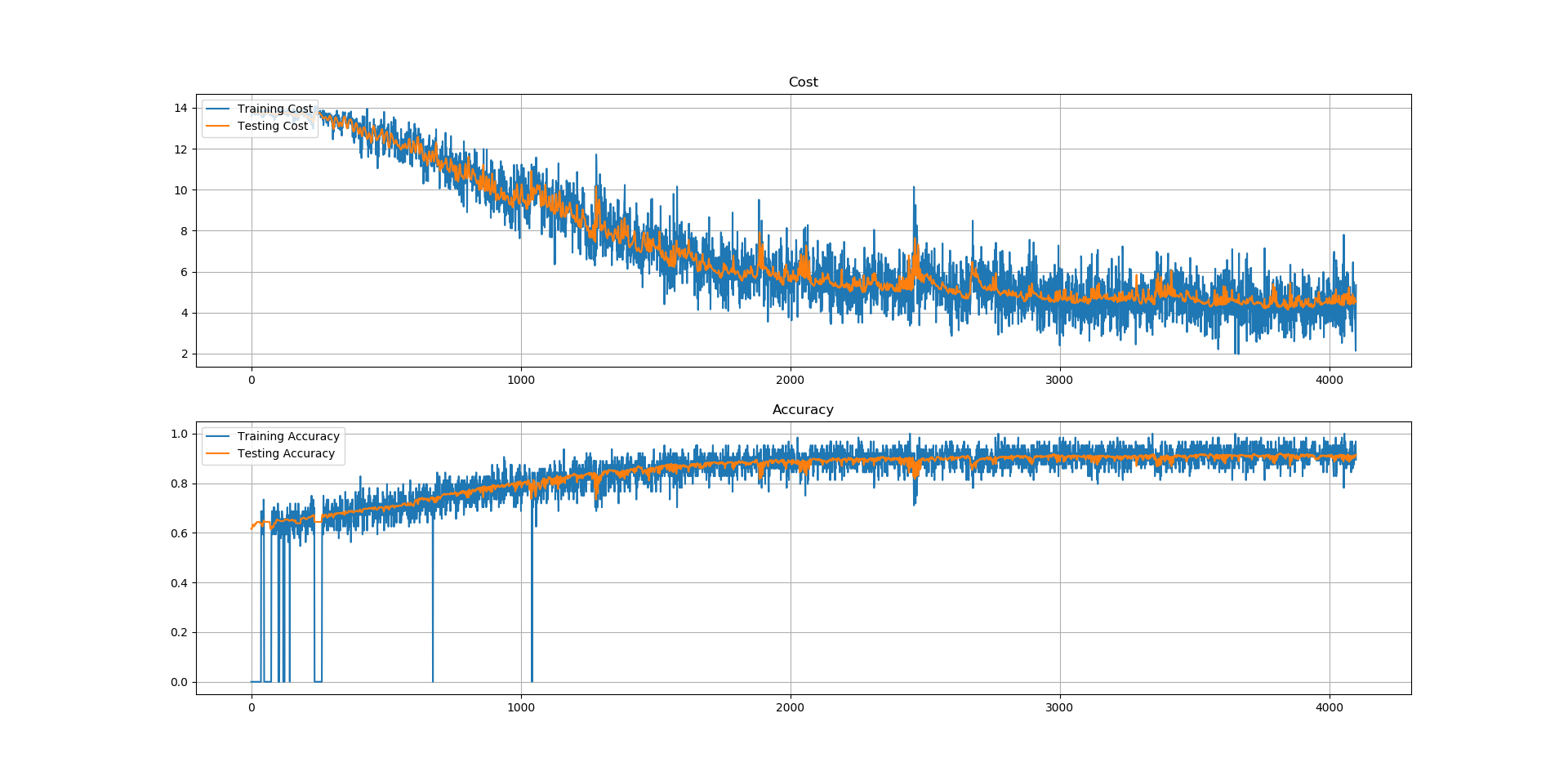
14-14x28-4 net |
1.166 | 3.10 | 0.9736 | 0.9340 |
The three following figures, show respectively
the cost and the accuracy for the 14-100-40-4 net, 14-28x6-4 net,
14-14x28-4 net architectures over the iterations 6.
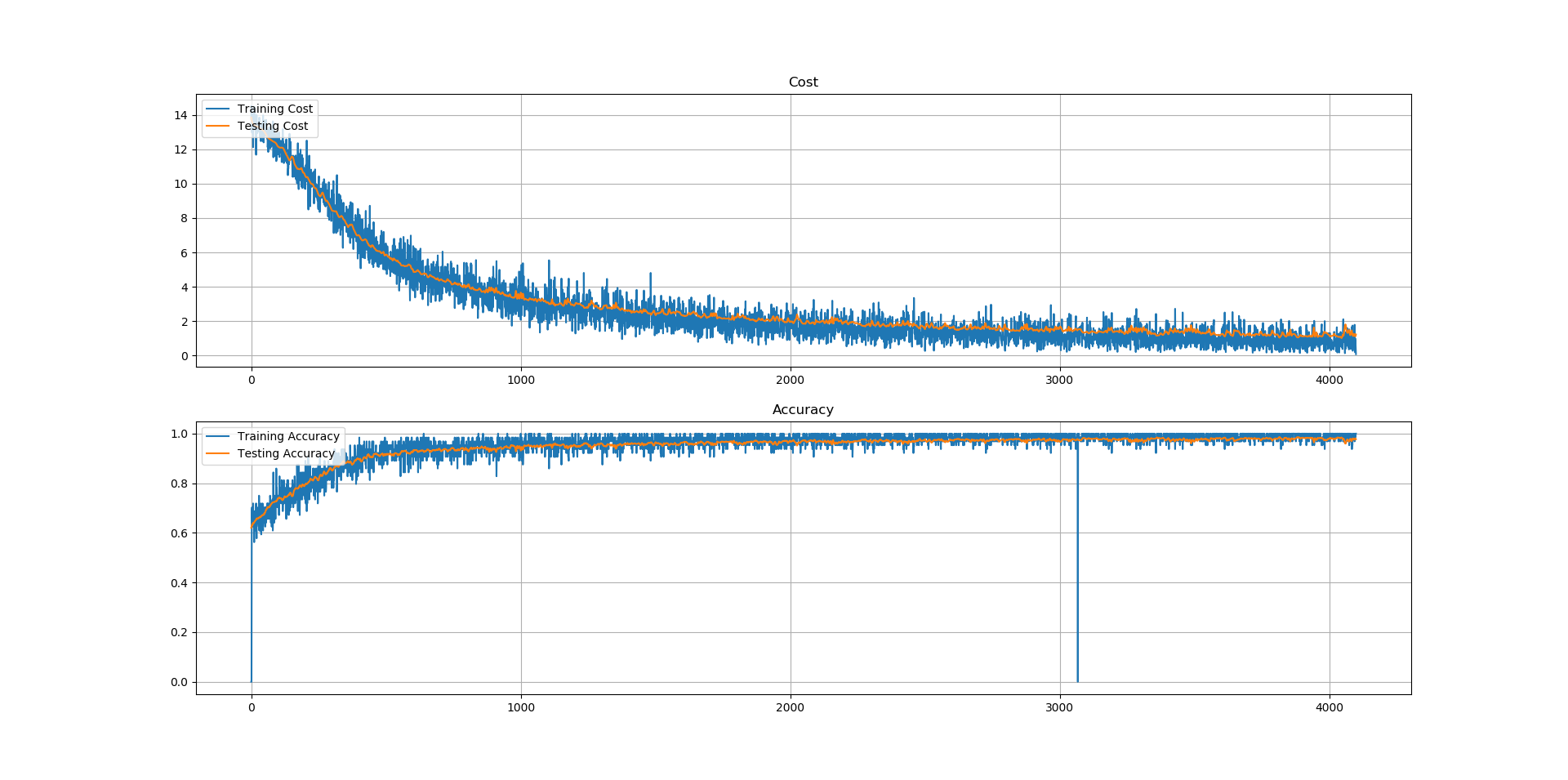
Indeed, using the entire dataset would give a better estimate of the cost $H$ and thus a good gradient and a hopefully (and idealy monotonically strictly) decreasing training cost. But this is computational demanding, and generally faster computations are preferred even if they do not give the best results: on the other hand, one sample at the time can be used to get faster computations, but this would give a really poor estimate of the cost function; thus resulting in having gradients that are not colinear to the real gradients of the cost (i.e. the one pointing to the steepest direction). Using mini-batches is in between those two approaches, namely Batch Gradient Descent (that uses the entire set) and Stochastic Gradient Descent (that uses only one random sample): it is still quite fast (as fewer example get evaluated instead of all the examples of the training set) but a reasonably good estimate of the cost can be obtained (thus resulting in a generally decreasing cost) that is definitively better than in SGD. Hence, this explains the irregular training costs and accuracies observed for the three architectures.
Moreover, the shallowest architectures are also the ones that are the easiest
to train: the first 14-100-40-4 net has a every iteration a better
accuracy than the second 14-28x6-4 net; the same observation between
the second and the last 14-14x28-4 net holds. Some parameters tuning
has been needed for the last architecture.
Finally, for the three architectures the testing accuracies seem to follow their associated training accuracies: this means that new example are as likely to be correctly classified as examples that are used to train those architectures. However, those claims should be verified: it might be possible that the testing accuracy drop after more epochs, meaning that the network would overfit the data.
In brief
In this article — that I would have wanted it to be shorter — we have seen the
base foundation of multilayer perceptron and its optimisation procedure.
joml has
also been presented as a way to see how could such networks be implemented minimalistically.
Bonus Track — Equivalence of two Neural Networks
Two networks are said to be equivalent if, they have the same number of input and output nodes, for all inputs, the outputs of both networks are identical. Given two neural networks as shown below, all activation functions $\sigma$ are identity functions:
$$ \sigma : z \mapsto z $$
Let’s say that we are here given a neural network $\mathcal{N}_A$ of three hidden layers; we thus have the following pairs of parameters:
$$ (W^{(0,1)},\, b^{(1)}), (W^{(1,2)},\, b^{(2)}), (W^{(2,3)},\, b^{(3)}) $$
Each layer has the same size and the same activation fonction defined to be the identity function, i.e:
$$ \left\{ \begin{matrix} &\forall l \in {1, \cdots,L},& N_l &=& N &=& 5\\ &\forall l \in {1, \cdots,L},& \sigma_l &=& \sigma &=& \text{Id}_{\mathbb{R}^N} \end{matrix} \right. $$
We want to construct an equivalent network $\mathcal{N}_B$ consisting of a simple layer having a single pair of parameters:
$$ (W,b) $$
$\mathcal{N}_A$ and $\mathcal{N}_B$ are equivalent, if they share the same number of inputs and outputs and if they give the same output for an identical input, i.e:
$$ \forall x \in \mathbb{R}^{N_0}:\quad \mathcal{N}_A(x) = \mathcal{N}_B(x) $$
The following values hold for all $x$: $$ \left\{ \begin{matrix} \mathcal{N}_A (x) &=& \sigma\left(W^{(2,3)}\,\sigma\left(W^{(1,2)}\,\sigma\left(W^{(0,1)}\,x + b^{(1)}\right) + b^{(2)}\right) + b^{(3)}\right)\\ \mathcal{N}_B (x) &=& \sigma\left(Wx + b\right) \end{matrix} \right. $$
As $\sigma = \text{Id}_{\mathbb{R}^N}$:
$$ \left\{ \begin{matrix} \mathcal{N}_A (x) &=& \left(W^{(2,3)}\,\left(W^{(1,2)}\,\left(W^{(0,1)}\,x + b^{(1)}\right) + b^{(2)}\right) + b^{(3)}\right)\\ \mathcal{N}_B (x) &=& Wx + b \end{matrix} \right. $$
Distributing products, we finally get: $$ \left\{ \begin{matrix} \mathcal{N}_A (x) &=& W^{(2,3)}\,W^{(1,2)}\,W^{(0,1)}\,x + W^{(2,3)}\,W^{(1,2)} b^{(1)} + W^{(2,3)}\,b^{(2)} + b^{(3)}\\ \mathcal{N}_B (x) &=& Wx + b \end{matrix} \right. $$
Thus, by identifying the terms, we get:
\begin{equation} \left\{ \begin{matrix} W& = &W^{(2,3)}\,W^{(1,2)}\,W^{(0,1)}\ b& = &W^{(2,3)}\,W^{(1,2)} b^{(1)} + W^{(2,3)}\,b^{(2)} + b^{(3)} \end{matrix} \right. \end{equation}
If the weights and biases are given in the first network with two hidden layers, we can write a program to find the weights and biases of the second network with no hidden layers to make the two networks equivalent.
References
- Yes. ↩
- See this Stack Exchange thread for a quick overview ↩
- See the original article: Adam: A Method for Stochastic Optimization ↩
- This is done per pair $(x^{(i)}, y^{(i)})$, but we do not indicate it here for the sake of notation. ↩
- Actually, means of gradients associated to each pair $(x^{(i)}, y^{(i)})$ are used for the updates, but again we do not indicate it here to make it readable. ↩
- An iteration is defined as the processing of one minibatch. ↩